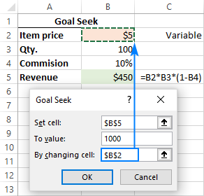
Set cell - the reference to the cell containing the formula B5. Use Goal Seek in Excel to find the grade on the fourth exam that produces a final grade of 70.

How To Use Goal Seek In Excel To Do What If Analysis

Goal Seek Example 1.

Goal seek analysis in excel 2013. The grade on the fourth exam in cell B5 is the input cell. In the Data tab click on what If Analysis. To value - the formula result you are trying to achieve 1000.

In the Set cell box enter the reference for the cell that contains the formula that you want to resolve. The goal seek function part of Excels what-if analysis tool set allows the user to use the desired result of a formula to find the possible input value necessary to achieve that result. You can think of it as some sort of a reverse tool wherein you have the desired result but you dont have the right value to get at that result.

This guide will focus on the goal seek command. In the Set cell box enter the reference for the cell that contains the formula that you want to resolve. Goal Seek is a built-in tool in Excel that would help you find the right value to get your desired result.

The Goal Seek dialog box appears. The Goal Seek dialog box will be. Move to cell B2 type the formulaA2A2-2A2-3 press to stay in B2 then double click on the cell handleto fill down the values - you should have values from 32 to 12 To see exactly whats happening plot the data on a graph.

Select the cell that contains your results formula. Before using any one. Type the amount you want the formula to return.

From What if Analysis select Goal Seek. Excel 2013 goal seek solver equation solution. The cell must contain a formula for Goal Seek to work To value.

A clip from Mastering Excel Made Eas. Open a work sheet and select a cell for which we want to use the Goal Seek function. Select the cell whose value you want to change.

In the Goal Seek dialog box fill out the criteria for your search. Curious what goal seek does. Other commands in the what-if analysis tool set are the scenario manager and the ability to create data tables.

In this case we would like a monthly payment of 600. A Goal Seek is a tool that is used to find an unknown value from a set of known values. On the Data tab in the Data Tools group click What-If Analysis and then click Goal Seek.

From the Data tab click the What-If Analysis command then select Goal Seek from the drop-down menu. The formula in cell B7 calculates the final grade. Sometimes when doing what-if analysis you have a particular outcome in mind such as a target sales amount or growth percentage.

This function instantly calculates the output when the value is changed in the cell. A dialog box will appear with. In the example this reference is cell B4.

On the Data tab select Goal Seek from the What-if Analysis dropdown menu. In the To value box type the formula result that you want. Whenever you use Goal Seek youll need to select a cell that already.

It comes under the What If Analysis feature of Microsoft Excel which is useful to find out the value that will give the desired result as a requirement. Go to the Data tab Forecast group click the What if Analysis button and select Goal Seek In the Goal Seek dialog box define the cellsvalues to test and click OK. In the example this reference is cell B4.

Press to select all the data or drag through cells A1to B12 7. On the Data tab in the Forecast group click What-If Analysis. Microsoft Excel 2013 Goal Seek and Solver Author.

When you need to do analysis you use Excel 2013s Goal Seek feature to find the input values needed to achieve the desired goal. Goal Seek Function in Excel 2013 Step 1. Normally the result is what you have to find from the data set.

Goal Seek in Excel 2013 Hi All I am having a bit of a problem with Goal Seek in Excel 2013It seems whenever i run the goal seek function the answer it returns is incorrect when i check it by inputting the value in manually and in addition the goal seek function removes the formula in the Set Cell and not even clicking the undo button restores it. In the To value box type the formula result that you want. On the Data tab in the Data Tools group click What-If Analysis and then click Goal Seek.

Find out now because it can save you time. To use Goal Seek example 1.

A box and whisker plot is a great tool to display the numerical summary of your data. However previous versions of Excel do not have it built-in.

Create A Box And Whisker Excel 2016 Myexcelonline

You can only inveigle a type of Excel chart into boxes and whiskers.

Excel box and whisker. Include the data label to selection so that it can be recognized automatically by Excel and it will be easier to modify and visualize the data. Any data point that falls outside the top or bottom whisker line would be considered an outlier when analyzing the data. The Box and Whisker Plot or Box Plot is a wonderful method of visually displaying the distribution of data through their quartiles minimum and maximum value.

To reverse the chart axes right-click on the chart and click Select Data. The whiskers on a box and whisker box plot chart indicate variability outside the upper and lower quartiles. They show you the distribution of a data set showing the median quartiles range and outliers.

In this article we are about to see how a Box-Whisker plot can be formatted under Excel 2016. In Excel a box and whisker chart also named as box plots is used to display the statistical analyses which helps to show you how numbers are distributed in a set of data. Box and Whisker Plot is an added graph option in Excel 2016 and above.

Select all the data from the third table and click Insert Insert Column Chart Stacked Column. The Box and Whisker chart was invented by John Tukey in 1977. Basically Excel does not offer Box and Whisker charts.

You dont have to sort the data points from smallest to largest but it will help you understand the box and whisker plot. For example select the range A1A7. This graph presents information from a five-number summary.

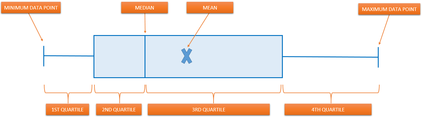
Simple Box and Whisker Plot. The line through the center is the median. Instead of showing the mean and the standard error the box-and-whisker plot shows the minimum first quartile median third quartile and maximum of a set of data.

These lines indicate variability outside the upper and lower quartiles and any point outside those lines or whiskers is considered an outlier. The whiskers go from each quartile to the minimum or maximum values. The Median divides the box into the interquartile range.

This example teaches you how to create a box and whisker plot in Excel. Choose the Plus direction select Custom for Error Amount and click on Specify Value. At first the chart doesnt yet resemble a box plot as Excel draws stacked columns by default from horizontal and not vertical data sets.

The Box and Whisker plots shows the median first quartile third quartile minimum and the maximum data set instead of showing mean and standard error. You can make and personalize your personalized evaluation in minutes when you make use of an box and whisker plot excel template. In this article we will learn how to create a box and whiskers chart in excel.

In a Box and Whisker chart numerical data is divided into quartiles and a box is drawn between the first and third quartiles with an additional line drawn along the second quartile to mark the median. Insert a box-and-whisker chart in Excel Start by selecting your data in Excel. The minimums and maximums outside the first and third quartiles are depicted with lines which are called whiskers.

Since then it is being used in statical plotting and graphing. In the box and whisker plot the lower box edge corresponds to the first quartile and the upper box edge corresponds to the third quartile. A box and whisker plot shows the minimum value first quartile median third quartile and maximum value of a data set.

Select the top box on the chart and then select Add Chart Element on the Chart Design tab. How to use Excel Box and Whiskers Chart. You can share as well as release your custom evaluation with others within your firm.

Box and Whisker Plots Excel. Box Whisker Plot in Excel is an exploratory chart used to show statistical highlights and distribution of the data set. Activate the Insert tab in the Ribbon and click on the Insert Statistics Chart icon to see the chart types under category.

The X in the box represents the Mean. Making Use Of box and whisker plot excel template for Excel worksheets can help boost performance in your service. What is a Box Plot.

The five-number summary is the minimum first quartile median third quartile and maximum. This chart is used to show a five-number summary of the data. In Excel you can make one in seconds.

These five-number summary are Minimum Value First Quartile Value Median Value Third Quartile Value and Maximum Value. To add the up whisker select the 3Q Box seriesthen in the Chart Tools Layout tab click Error Bars and select More Error Bar Options from the bottom of the menu. The boxes may have lines extending vertically called whiskers.

A box and whisker chart shows distribution of data into quartiles highlighting the mean and outliers. Box and Whisker Excel is one of the many new Charts available only in Excel 2016 and was originally invented by John Tukey in 1977. Instead you can cajole a type of Excel chart into boxes and whiskers.

The graph was initially called Boxplot. Excel doesnt offer a box-and-whisker chart. The Box and Whiskers chart is used in analytics to visualise mean median upper bound and lower bound of a data set.

For example click any cell in row 4 to freeze rows 1 2. Click the Freeze Panes command.

Freeze Panes In Excel 2010

Cells above and to the left of the current cell will be frozen.

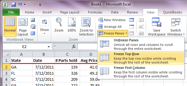
Excel 2010 freeze panes. Select View Freeze Panes Freeze Panes. Excel will Freeze Panes in an unpredictable way in which you did not intend. This will freeze Row 1 and Column A so that as you scroll through your worksheet you will always be able to see the titles across the top and the data in column A.

To freeze one row only click Freeze Top Row. Start by selecting the row below the last row you want to freeze. Using Freeze Panes Select the First row or First Column or the row Below which you want to freeze or Column right to area which you want.

Press F to freeze both rows and columns in excel based on where your cursor is this will freeze rows and columns to the right and to the left of your cursor Press R to freeze the top row in excel only. Choose Page Layout command and this will undo any frozen panes that you have in place. In the View tab click Freeze Panes and select the freeze option you want to use.

To freeze one column only click Freeze First Column. Press C to freeze the first column in excel only. For example if you wish to lock the top two rows place the mouse cursor in cell A3 or select the entire row 3.

For example choose Freeze top row to freeze the top row. For example if you want columns A and B to always appear to the left of the worksheet even as you scroll select column C. You can use the Alt-W-F shortcut to enable the Freeze Panes options.

To fix this click View Window Unfreeze Panes. Freeze Top Row To freeze first row of worksheet. Excels Freeze Panes command also becomes disabled when the workbook is protected in Excel 2010 and earlier as illustrated in Figure 2.

Follow answered Dec 20 18 at 1609. Head over to the View tab and click Freeze Panes Freeze Panes. To freeze the first column execute the following steps.

Click the View tab. Restore lost frozen panes by selecting Page Layout view. To rectify this Ringstrom suggests.

Excel 2010 Freeze Panes. Click View - Freeze Pane - Freeze Top row or Freeze Top Coll. Then click on the Unfreeze Panes option in the popup menu.

Select the column to the right of the columns you want frozen. Due to changes with how windows are containerized in Excel 2013 and later you no longer protect Windows in those versions when protecting a workbook. Youre scrolling down your worksheet or scrolling to the side but part of it is frozen in place.

Select the suitable option Freeze Panes To freeze area of cells. Freeze Panes in Excel VBA Similar to freeze panes in Excel spreadsheet to freeze panes in Excel VBA select a Cell first then set ActiveWindowFreezePanes Property to TRUE. Freeze Slicers in excel 2010.

This is probably because at some point you decided to freeze the panes. Freeze rows or columns Select the cell below the rows and to the right of the columns you want to keep visible when you scroll. Choose either Normal or Page Break Preview commands to enable the Freeze panes.

Then there are three options. For example click any cell in column B to. On the View tab in the Window group click Freeze Panes.

How to Hide the Freeze Panes Line. Then make the row or column as big as you need to fit your slicers in. Click the View tab.

Choose View Tab Freeze Panes. Say you select Freeze Panes when the three rows that you are attempting to freeze are scrolled off the sheet view. Select the View tab from the toolbar at the top of the screen and click on the Freeze Panes button in the Windows group.

To freeze more than one row or column or to freeze both rows and columns at the same time click Freeze Panes. Select the row below the rows you want to freeze. Select the column to the right of the columns you want to freeze.

Ask Question Asked 2 years 1 month ago. Note the lines indicating that rows and columns above and to the left of I12 are frozen. Freezing panes could hide rows or columns or cause the column headings to always be visible even after scrolling.

To unfreeze panes open your Excel spreadsheet. Freeze Both Top Row and Left Column A If you want to freeze both the top row and column A select cell B2 and go to ViewFreeze PanesFreeze Panes.

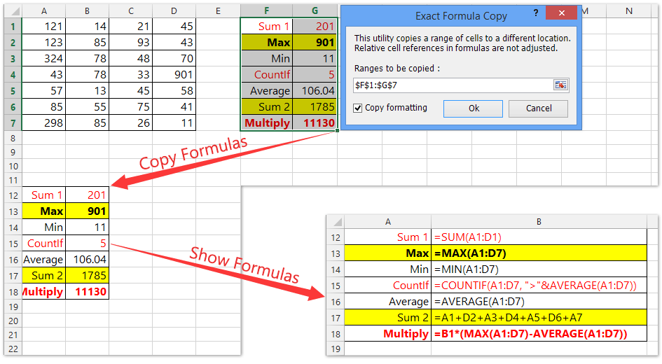
For example cell A3 below contains the SUM function which calculates the sum of the range A1A2. This formula glues together the pieces of text that appear in B4 C4 and D4 using the ampersand which is the concatenation operator in Excel.

How To Insert Function In Excel Top 2 Methods To Insert Formulas

Enter a number in cell A1.

Entering formulas in excel. Normally if you try to enter a formula in an unfinished state Excel will throw an error stopping you from entering the formula. If you dont type the equals sign first then Excel will assume you are typing either a number or a text. Greater than or equal to.

The formula string must start with an equal sign after the first quotation mark. This setting can be changed by macros or by other workbooks that you may have opened first. Change it to Automatic and the formulas will start working.

Type Shift8 on the top row of the keyboard. How to create Excel math formulas and how to refer to other cells from w. In Excel IF formulas you are not limited to using only one logical function.

Is not equal to. The formula below does the trick. To see how altering one of the formula values alters the result change the data in cell C1 from 3 to 6 and press Enter on your keyboard.

To increase the number in cell A1 by 20 multiply the number by 12 102. We get the results below. The result appears in cell E1.

If this is set to manual the formulas will not update unless you press the Calculate Now or Calculate Sheet buttons. Press Enter to complete the formula. When entering a formula you have to make sure Excel knows thats what you want to do.

When you click AutoSum Excel automatically enters a formula that uses the SUM function to sum the numbers. You start by typing the equals sign then the rest of your formula. Select a cell next to the numbers you want to sum click AutoSum on the Home tab press Enter Windows or Return Mac and thats it.

Excel will then display a hint pop-up for that function that shows all arguments. This action places the cell reference B2 in the formula. When inputting true or false conditions of an IF-THEN statement in Excel you need to use quotation marks around any text you want to return unless youre using TRUE and FALSE which Excel automatically recognizes.

To select arguments easily click in the function in the Formula Bar or cell whose argument you want to select. Select cell B2 in the worksheet by using the mouse or the keyboard. Example 3 Excel IF Statement.

IF OR AND formula in Excel. An equal sign. Here is a simple example of a formula in a macro.

Less than or equal to. Enter a decimal number 02 in cell B1 and apply a Percentage format. Here is an example of IF AND OR formula that tests a couple of OR conditions within AND.

Type a plus sign then use your pointer to select C2 to enter the second cell reference into the formula. A formula is an expression which calculates the value of a cell. The process usually starts by typing an equal sign followed by the name of an Excel function.

Select the next cell or type its address. In Column B we will use a formula to check if the cells in Column C are empty or not. The value of the formula must start and end in quotation marks.

Formulas in Excel always begin with the equal sign. Select a cell or type its address in the selected cell. In between each piece of text the CHAR function appears with the character code 10.

Typing a formula in a cell or the formula bar is the most straightforward method of inserting basic Excel formulas. However if you add a single apostrophe before the equal sign Excel will treat the formula as text and let you enter without complaint. Other values and formulas dont require quotation marks.

The character code for a line break in Excel varies depending on the platform. Excel displays the calculated answer in cell C2 and the formula A2B2 in the Formula bar. If a part of the formula is in parentheses that part will be.

This short video tutorial shows how to enter a simple formula into your Excel sheet. Create a formula that refers to values in other cells. A pop-up appears below the Formula Bar or below the cell.

Click the Formulas tab and then the Calculation Options button. Type the equal sign. For example cell A3 below contains a formula which adds the value of cell A2 to the value of cell A1.

Excel is quite intelligent in that when you start typing the name of the function a pop-up function hint will show. To check various combinations of multiple conditions you are free to combine the IF AND OR and other functions to run the required logical tests. The formula is a string of text that is wrapped in quotation marks.

You can also start a formula with either a plus or minus - symbol. Excel uses a default order in which calculations occur. Start by entering the formula with the function.

Functions are predefined formulas and are already available in Excel. For example for subtraction. If a cell is blank the formula will assign the status open However if a cell contains a date then the formula will assign a status of closed The formula used is.

The For loop is typically used to move sequentially through a list of items or numbers. You can use a single loop to loop through a one-dimensional range of cells.

Excel Vba Loops For Each For Next Do While Nested More Automate Excel

The For loop has two forms.

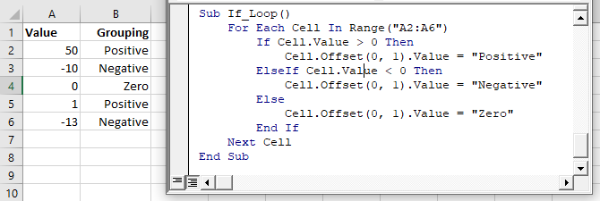
Excel vba for loop. The code compares each value of a cell in column A with that of column B. For next loop loops through the cells and perform the task and For Each loop loops through objects like Worksheets Charts Workbooks Shapes. In VBA Break For Loop is also known as exit for loop every loop in any procedure has been given som11e set of instructions or criteria for it to run nuber of time but it is very common that some loop get into an infinite loop thus corrupting the code in such scenarios we need break for or exit for loop to come out of certain situations.

There may be any number of loops within a loop but the loops has to be properly nested without any conflict. Next loop and the For Each loop. Here is a simple example of using VBA loops in Excel.

If it turns out to be even you give it a color else you leave it as is. This feature of Excel is very useful in comparing a range of cells and is most often used in Excel Programming. For Next and For Each In Next.

For Loop is sometimes also called For Next Loop. The Microsoft Excel FORNEXT statement is used to create a FOR loop so that you can execute VBA code a fixed number of times. There are 4 basic steps to writing a For Each Next Loop in VBA.

VBA Break is used when we want to exit or break the continuous loop which has certain fixed criteria. Suppose you have a dataset and you want to highlight all the cells in even rows. The For Each loop as compared to the For loop cant be used to iterate from a range of values specified with a starting and ending value.

Add line s of code to repeat for each item in the collection. MyString MyString Chars Append number to string. A VBA For Loop is best used when the user knows exactly how many times the loop process needs to repeat.

The VBA For Loop Introduction The For Loop in combination with the If Statement unlocks a lot of the coding potential in VBA. In VBA loops allow you to go through a set of objectsvalues and analyze it one by one. In many of the examples up to this point we have been either looking at single cells and performing testsoperations on those single cells or we have been explicitly referencing multiple cells.

Instead you can specify a collection of objects and it will be able to loop through all those objects one by one. A loop in Excel VBA enables you to loop through a range of cells with just a few codes lines. Dim Words Chars MyString For Words 10 To 1 Step -1 Set up 10 repetitions.

The outer loop uses a loop counter variable that is decremented each time through the loop. Next Chars Increment counter MyString MyString Append a space. The VBA code inside the loop is then executed for each value.

You can use a VBA loop to go through the range and analyze each cell row number. How to declare a For Each Loop. This process can be performed using the do until or do while.

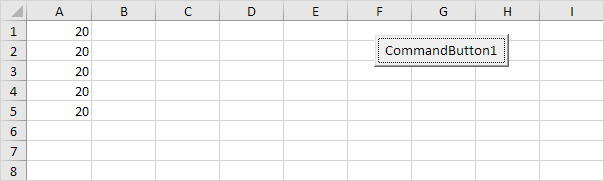
Place a command button on your worksheet and add the following code lines. The following example illustrates the nested loop. The Loop Builder allows you to quickly and easily build loops to loop through different objects or numbers.

If you want to loop through all the cells from a range. The VBA For Each loop is a scope that defines a list of statments that are to be repeated for all items specified within a certain collectionarray of items. The For Loop in VBA is one of the most common types of loop.

These are the For. Write the For Each Line with the variable and collection references. For loop is one of the most important and frequently used loop in VBA.

The criteria set in the for loop automatically creates a counter variable and will add 1 to the loop until the counter reaches the last value. Declare a variable for an object. In the For Each Next you dont need to specify the count of iterations.

Following is the syntax of a for loop in VBA. To end the For loop at any given point we can use the exit statement. VBA For Loop Example 3 Find the last row with data Store the value in variable Use the variable to determine how many times the loop runs.

Next loop uses a variable which cycles through a series of values within a specified range. VBA FOR EACH NEXT is a fixed loop that can loop through all the objects in a collection. You can also perform specific tasks for each loop.

The FORNEXT statement is a built-in function in Excel that is categorized as a Logical Function. It can be used as a VBA function VBA in Excel. Sometimes when we use any loop condition in VBA it often happens that the code keeps on running without an end or break.

For counter start To end Step stepcount statement 1 statement 2. You can perform actions on each object andor select only objects that meet certain criteria. VBA Loop Builder This is a screenshot of the Loop Builder from our Premium VBA Add-in.

Syntax of VBA For Loop. Type 2 For Each Loop For Each loop in VBA is for looping through a collection of objects. For Chars 0 To 9 Set up 10 repetitions.

For loop is within the scope range defines the statements which get executed repeatedly for a fixed number of time. The Visual Basic For loop takes on two separate forms. For Loop will go round and round until it meets the end condition.

Using this loop we can go through all the worksheets and perform some tasks. For Loops allow you to iterate a set of statements for a specified number of times. This is best explained by way of a simple example.

Looping is one of the most powerful programming techniques. Statement n Exit For statement 11 statement 22.