Excel 2010 Conditional Formatting Accross multiple tables. Select the data range containing the invoice values click on Conditional Formatting available on Home tab.

Excel Conditional Formatting Formulas

You can use the search option to highlight specific cells in.

Conditional formatting excel 2010 based on another cell. Excel Conditional Formatting Entire Row Based on One Cell Text. Once you click on that option it will open a new window for you. Select the cells you want to format.

Create a conditional formatting rule and select the Formula option. To do this select the range of cells that you wish to apply the conditional formatting to. Enter the value 60 and select any formatting style.

Excel Conditional Formatting Based on Another Cell Value Step 1. Then in the Styles group click on the Conditional Formatting drop-down and select Manage Rules. Excel conditional formatting based on another cell text 5 ways Highlighting Cells Based on Another Cell Text with Formula.

But this is a delusion. Criteria 1 Text criteria. How to change cell colour based on previous cell data.

Select the first cell in the first row youd like to format click the Conditional Formatting button in the Styles section of the Home tab and then select Manage Rules from the dropdown menu. Conditional Formatting specific cells based on their values as well as value in another cell. How to use Conditional Formatting Based On Another Cell Value.

Enter a formula that returns TRUE or FALSE. You can create a formula-based conditional formatting rule in four easy steps. Auto strikethrough based on cell value with Conditional Formatting Auto strikethrough based on cell value with Conditional Formatting In fact the Conditional Formatting feature in Excel can help you to finish this task as quickly as you can please do as this.

Yepyou can conditionally format a cell based on the value of a cell in a different worksheet by referencing the sheet name in the formula. Criteria 2 Number criteria. Then select the Home tab in the toolbar at the top of the screen.

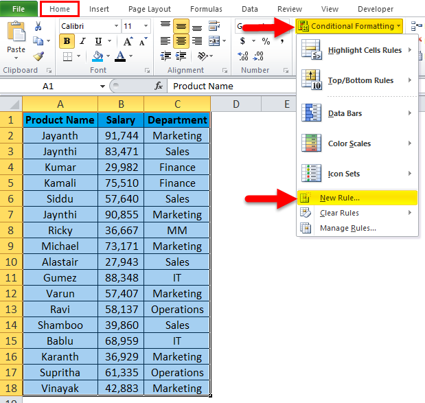
In order to achieve this we need to follow the below steps. We can highlight an excel row based on cell values using conditional formatting using different criteria. Navigate to Home tab and click Conditional Formatting button you will see list of different options.

In the list box at the top of the dialog box click the Use a Formula to Determine which Cells to Format option. Excel contains many built-in presets for highlighting values with conditional formatting including a preset to highlight cells greater than a specific value. A common opinion is that Excel conditional formatting icon sets can only be used to format cells based on their own values.

The ISODD function only returns TRUE for odd numbers triggering the rule. Apply conditional formatting based on values in another column Supposing you have a table as the below screenshot shown and want to highlight cells in column B if the adjacent cell values in column C are greater than 800 please apply the Conditional Formatting function as follows. Choose the rule type Format only cells that contain.

Select the entire data. In the Conditional Formatting Rules Manager window click the New Rule button. For example instead of A1 you would use Sheet1A1.

Select the data cells in your target range cells E3C14 in this example click the Home tab of the Excel Ribbon and then select Conditional FormattingNew Rule. With just a little creativity you can assign icons depending on the values of other cells in a row or based on another cells value as demonstrated in the following examples. Lets say you want to highlight the names of.

For example if you want to apply conditional formatting using a condition that If a cell value is greater than a set value say 100 then format the cell as RED else format the cell as GREEN. Create a conditional formula that results in another calculation or in values other than TRUE or FALSE Create a conditional formula that results in a logical value TRUE or FALSE To do this task use the AND OR and NOT functions and operators as shown in the following example. Criteria 4 Different color based on multiple conditions.

However by using your own formula you have more flexibility and control. Go to Home Conditional Formatting Highlight Cells Rules Text That Contains. This opens the New Formatting Rule dialog box.

In this example weve selected cells E14 to E16. Criteria 3 Multiple criteria. Set formatting options and save the rule.

In this window mention the text value that. Choose New Rule from the drop-down menu. Select the Marks column go to conditional formatting and in Highlight Cells Rules click Less than.

The sheet name must be enclosed in single quotes if it contains a space for example Sheet 1A1. So you can see that it requires two rules to perform the conditional formatting one for greater than 100 and one for less than 100.

Select Containing beside it and write Blue after that. Conditional format based on another cell value In the example above we are changing the cell color based on that cell value only we can also change the cell color based on other cells value as well.

Conditional Formatting Based On Another Cell Learn How To Apply

From the Format Rules section select Custom Formula.

Conditional format based on another cell. Select the entire data. Perform Conditional formatting based on another cell value in excel In this article we will learn about how to use Conditional formatting based on another cell value in Excel. C5 J6.

Now select the New Rule from Conditional Formatting option under the Home tab. Then format the cells with a format you need. The Apply to Range section will already be filled in.

For example instead of A1 you would use Sheet1A1. Its a very easy process to set up a formatting formula. The process to highlight cells based on the date entered in that cell in Google sheets is similar to the process in Excel.

Select the text list that you want to highlight the cells which contain partial text and then click Home Conditional Formatting New Rule see screenshot. The sheet name must be enclosed in single quotes if it contains a space for example Sheet 1A1. In conditional formatting any number greater than 0 is considered True.

Once we click OK and apply the rule to the selected cells Excel will automatically format the cells whenever a user replaces a formula cell with a static cell value as shown below. Excel 2019 - Conditional Formatting specific cells based on their values as well as value in another cell. These cells can be duplicate values or they may fall within certain limits or a similar criteria.

First select the cells where you want to apply the conditional formatting. In todays tutorial we will be explaining how to highlight a cells value when it meets criteria in a cell. In the example shown the formula used to apply conditional formatting to the range C5G15 is.

No I want do Conditional Formatting of Sheet2 range A1M13 based on the cell values in Sheet1 A1M13 because I dont want text in the cell of Sheet2 so I can put in random text which doesnt effect cells background etc. In the list box at the top of the dialog box click the Use a Formula to Determine which Cells to Format option. In simple words We need to view highlighted data on the basis of values in another cell.

The process to highlight cells based on the text contained in that cell in Google sheets is similar to the process in Excel. This opens the New Formatting Rule dialog box. Highlight the cells you wish to format and then click on Format Conditional Formatting.

In this window mention the text value that. To conditional formatting between two dates select the cells and use this formula AND B2D2B2. First select the entire data from A3E13 as shown below.

If text is exactly 1 to 15 so 15 rules each number gives the cell a different background filling. Go to Home Conditional Formatting Highlight Cells Rules Text That Contains. How to build a search box with conditional formatting In this video well look at a way to create a search box that highlights rows in a table by using conditional formatting and a formula that checks several columns at once.

Go to the HOME tab. Excel Conditional Formatting Based on Another Cell Value Step 1. When we want to format a cell based on the value in a different cell we will use a formula to define the conditional formatting rule.

In this video well look at how to apply conditional formatting to one cell based on values in another using a formula. Yepyou can conditionally format a cell based on the value of a cell in a different worksheet by referencing the sheet name in the formula. To apply conditional formatting based on a value in another cell you can create a rule based on a simple formula.

In the New Formatting Rule dialogue box select Format only cells that contain and in the Format only cells with option select Specific Text. Here the formula is COUNTBLANK B2D2. From the Format Rules section select Custom Formula and type in the formula.

The Apply to Range section will already be filled in. Conditional formatting values in a column based on other columns. Select the data cells in your target range cells E3C14 in this example click the Home tab of the Excel Ribbon and then select Conditional FormattingNew Rule.

Suppose we want to change the color of cell E3 based on the value in D3 to do that we have to use a formula in conditional formatting. Sheet1 has a range of cells A1M13 which have conditional format rules. We select the desired cell formatting by clicking the Format button.

Highlight the cells you wish to format and then click on Format Conditional Formatting. And that is the ISFORMULA and conditional formatting method to address the issue. The conditional formatting is used for highlighting cells that meet certain criteria.

Once you click on that option it will open a new window for you. How to change cell colour based on previous cell data. We have locked columns and left rows relative.

Conditional formatting based on date in another column. Here we have used the COUNTBLANK function that counts the number of blank cells in a range.